Statistics and probability

Data in everyday life

Statistics is the science of collecting, organizing, analysing and interpreting data. Election surveys, weather forecasts, class rankings and the price of rice all rest on it. A good statistician also asks whether the data can be trusted and whether a conclusion really follows from it.

Kinds of data

• Qualitative (categorical) data are labels: blood type, course, province.
• Quantitative data are numbers. They are discrete when they are counted (the number of siblings) and continuous when they are measured (height, time, weight).

Data also have a level of measurement: nominal (names only, such as jersey numbers), ordinal (ordered, such as 1st, 2nd and 3rd place), interval (equal steps but no true zero, such as temperature in °C) and ratio (equal steps and a true zero, such as weight or income).

Organizing data

A frequency table counts how often each value occurs. The quiz scores 7, 8, 8, 9, 7, 10, 8, 9, 8, 6 give:

From the table you can read the mode at once (8) and draw a bar graph or histogram.

Summarizing data

• Mean: the sum divided by the count. The mean of 4, 8, 6, 10, 12 is 40 ÷ 5 = 8.
• Median: the middle value in order, or the average of the middle two. For 3, 7, 9, 12, 15, 20, it is (9 + 12) ÷ 2 = 10.5.
• Mode: the most frequent value.
• Range: highest minus lowest.
• Variance and standard deviation: how far values spread around the mean. The standard deviation is the square root of the variance.

Choosing a measure of centre

The mean uses every value, so one extreme value pulls it. If five employees earn ₱20,000, ₱22,000, ₱21,000, ₱23,000 and ₱150,000, the mean is ₱47,200, which describes nobody. The median, ₱22,000, is more typical. Use the median when the data are skewed or have outliers, the mean when they are roughly symmetric, and the mode for categories such as the most popular course. A data set can have no mode, one mode, or several.

The weighted mean

When values count for different amounts, multiply each by its weight, add, and divide by the total weight:

weighted mean = Σ(x × w) ÷ Σw

A college GWA is a weighted mean, with the units of each subject as weights. A student earns 1.5 in a 3-unit subject, 2.0 in a 5-unit subject and 1.25 in a 2-unit subject. The total is 1.5 × 3 + 2.0 × 5 + 1.25 × 2 = 4.5 + 10 + 2.5 = 17, over 10 units, so the GWA is 17 ÷ 10 = 1.7. The ordinary mean of the three grades, about 1.58, ignores the units and is wrong.

Measuring spread

The range uses only two values. The standard deviation uses all of them. For a population, subtract the mean from each value, square the differences, average the squares to get the variance, and take the square root.

For 2, 4, 4, 4, 5, 5, 7, 9 the mean is 40 ÷ 8 = 5. The differences from 5 are −3, −1, −1, −1, 0, 0, 2 and 4, and their squares add up to 9 + 1 + 1 + 1 + 0 + 0 + 4 + 16 = 32. The variance is 32 ÷ 8 = 4 and the standard deviation is √4 = 2. For a sample, divide by n − 1 instead of n, which gives a slightly larger value.

A small standard deviation means the values cluster near the mean; a large one means they are scattered. Two classes can both average 80 while one has scores from 78 to 82 and the other from 50 to 100.

Quartiles and position

The median splits ordered data in half. The quartiles split it into quarters: Q₁ has a quarter of the data below it, Q₂ is the median, and Q₃ has three quarters below it. A percentile works the same way in hundredths, so a score at the 90th percentile beat about 90% of the group.

1. The normal curve

In a normal distribution, about 68% of values lie within 1 standard deviation of the mean, about 95% within 2, and about 99.7% within 3.

A z-score counts standard deviations from the mean: z = (x − mean) ÷ SD. A score of 85 with mean 75 and SD 5 has z = 2.

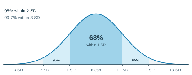
The normal curve is bell-shaped and symmetric, and its mean, median and mode are equal. Many measurements, such as heights, exam scores and measurement errors, are close to normal. If the heights of a group of students are normal with mean 160 cm and SD 6 cm, about 68% are between 154 and 166 cm and about 95% are between 148 and 172 cm.

Because the curve is symmetric, half of each band lies on either side of the mean. So about 34% lie between the mean and 1 SD above it, and about 2.5% lie more than 2 SD above it. A negative z-score is below the mean: a height of 151 cm has z = (151 − 160) ÷ 6 = −1.5. Z-scores let you compare results from different tests, because they measure position in standard deviations rather than raw points.

2. Sampling

A population is the whole group we want to know about; a sample is the part we actually measure. A number that describes a population is a parameter; one that describes a sample is a statistic.

• Simple random: everyone has an equal chance, as in a lottery.
• Systematic: every kth name on a list.
• Stratified: a random sample from each subgroup.
• Cluster: randomly chosen whole groups, such as sections.

Asking only your friends, or only people who answer an online poll, is convenience sampling. It is cheap but biased, because the people who are easy to reach may not represent everyone.

How large a sample? Slovin’s formula

Slovin’s formula gives a sample size n for a population of size N and a margin of error e:

n = N ÷ (1 + Ne²)

Always round up, since rounding down would give a larger error than allowed. For a town of 10,000 people with a 5% margin, e = 0.05 and e² = 0.0025, so n = 10,000 ÷ (1 + 25) ≈ 384.6, and you survey 385 people. A smaller margin needs a much larger sample.

3. Relationships between variables

Statistics also asks whether two variables move together. Correlation measures how closely paired data follow a straight line, using Pearson’s r, which runs from −1 to 1. A value near 1 means a strong positive link (more study hours, higher scores), near −1 a strong negative link, and near 0 no linear link. A regression line uses the link to predict one variable from the other. Correlation does not prove causation: ice cream sales and drownings both rise in summer, but neither causes the other.

4. Probability

P(event) = favourable outcomes ÷ possible outcomes. On a fair die, P(greater than 4) = 2/6 = 1/3. For independent events, multiply: two heads in two tosses is 1/2 × 1/2 = 1/4.

The set of all possible outcomes is the sample space. A probability is always between 0 (impossible) and 1 (certain), and the probabilities of all outcomes add up to 1.

• Complement: P(not A) = 1 − P(A). The probability of not rolling a 6 is 1 − 1/6 = 5/6.
• Addition rule: P(A or B) = P(A) + P(B) − P(A and B). From a standard deck of 52 cards, P(heart or king) = 13/52 + 4/52 − 1/52 = 16/52 = 4/13. The king of hearts is subtracted once because it was counted twice, exactly as in the overlap rule for sets.
• Mutually exclusive events cannot happen together, so P(A and B) = 0 and their probabilities simply add.

Solved examples

Follow each one line by line. The steps stay the same when the numbers change, so cover the steps and try it yourself.

Example 1: Mean, median, mode and range

Question: Find the mean, median, mode and range of 6, 10, 3, 10, 16.

1. Sort first. 3, 6, 10, 10, 16.
2. Mean: add, then divide by the count. 45 ÷ 5 = 9.
3. Median: take the middle of the sorted list. The 3rd of 5 values is 10.
4. Mode: find the most frequent. 10 appears twice.
5. Range: highest minus lowest. 16 − 3 = 13.

Answer: Mean 9, median 10, mode 10, range 13.

Example 2: z-score and the normal curve

Question: A test has mean 60 and SD 8. A student scores 76. What is the z-score, and about what percent of scores lie between 44 and 76?

1. Write the rule. z = (x − mean) ÷ SD.
2. Substitute. (76 − 60) ÷ 8 = 16 ÷ 8 = 2.
3. Count SDs on the other side. (44 − 60) ÷ 8 = −2, so the range runs from 2 SD below to 2 SD above the mean.
4. Use the 68–95–99.7 rule. Within 2 SD is about 95%.

Answer: z = 2, and about 95% of scores lie in that range.

Example 3: Probability of two independent events

Question: A bag has 3 red, 5 blue and 2 green marbles. One marble is drawn and a coin is tossed. What is the probability of green and heads?

1. Find the first probability. Green: favourable ÷ possible = 2 ÷ 10 = 1/5.
2. Find the second probability. Heads: 1/2.
3. Decide how to combine. The coin does not affect the marble, so the events are independent. Multiply.
4. Multiply. 1/5 × 1/2 = 1/10.

Answer: The probability is 1/10.

Common mistakes

• Finding the median of unsorted data. Put the values in order first.
• Using the ordinary mean for a GWA. Units are weights; multiply before you add.
• Rounding Slovin’s answer down. Always round the sample size up.
• Forgetting to halve the bands. 68% lie within 1 SD on both sides together; only 34% lie on one side.
• Double counting in "or". Subtract the outcomes that are in both events.
• Reading correlation as cause. A link between two variables may come from a third one.

Where you will meet this

• School records. GWAs, class standings and percentile ranks are weighted means and positions.
• Research. Theses use sampling methods, Slovin’s formula and correlation.
• News and elections. Survey results come with a margin of error from the sample size.
• Health and insurance. Risks and premiums are set from probabilities.

Key terms

Mean, median, mode

The average, the middle value in order, and the most frequent value.

Weighted mean

A mean in which each value is multiplied by its weight before dividing by the total weight.

Standard deviation

The square root of the variance; a typical distance of values from the mean.

z-score

The number of standard deviations a value lies above or below the mean.

Sample

The part of a population that is actually measured.

Sample space

The set of all possible outcomes of an experiment.

Summary

• Classify data first; it decides which summaries make sense.
• The mean uses every value, the median resists outliers, the mode suits categories, and a weighted mean uses weights.
• The standard deviation measures spread; z = (x − mean) ÷ SD measures position.
• On a normal curve, about 68%, 95% and 99.7% lie within 1, 2 and 3 SD of the mean.
• Choose a random sampling method, and size the sample with n = N ÷ (1 + Ne²), rounded up.
• P(not A) = 1 − P(A); P(A or B) = P(A) + P(B) − P(A and B); multiply for independent events.